Visualizing Graphs in Program Output
Many computer science problems utilize graph-based data structures. Their use can range from explicit inclusion in an algorithm-centric problem (like path-finding) to a more “behind-the-scenes” presence in Bayesian networks or descriptions of finite automata. Unfortunately, visualizing large graphs can be difficult to do, especially for debugging. Unlike lists or dictionaries, which can be represented clearly by plain text printing, depicting a graph tends to require more graphics overhead than is reasonable for most programmers to write simply for debugging purposes. I’ve found that Graphviz, a free graph visualization utility, can be quite useful in debugging graph-related programs.
Installing Graphviz
If you’re on a Debian-based Linux OS (e.g. Ubuntu), you can install Graphviz using apt-get. Just run $ sudo apt-get install graphviz and you’ll have everything you need to complete the steps in this blog post. Mac OS X users can use brew equivalently.
Windows users should install using a binary downloaded from the Graphviz Windows page, but there might be some issues with setting the PATH variable for running in the commandline.
Making a basic graph
Once you’ve installed, the next thing you’ll want to do is create a basic graph to ensure the installation succeeded and to gain practice using Graphviz tools. We do this by creating a *.dot file that describes the graph we wish to display. If you’re the type of person who likes to jump right in and experiment first before reading too much, or if you love formal language specification, the DOT grammar is fairly readable and can give a quick introduction to creating DOT files.
The below is a fairly representative DOT file to demonstrate some of the capabilities of Graphviz. Open your favorite text editor, copy/paste it in, and save it as firstgraph.dot:
 1digraph G {
 2  // Style information for nodes
 3  A [style="filled", color=".05 .3 1.0"]
 4
 5  // Edge declarations
 6  A -> {B, C};
 7  D -> E [label="-1"];
 8  E -> F [label="3"];
 9  F -> D [label="10"];
10}
This creates a directed graph (also called a digraph) with six nodes and two connected components. Some of the edges have labels, and one of the nodes is colored. After you’ve copied (or downloaded) this file, open up a terminal to the directory with firstgraph.dot in it and run $ dot firstgraph.dot -Tpng -o firstgraph.png. The resulting image file should look something like the below:
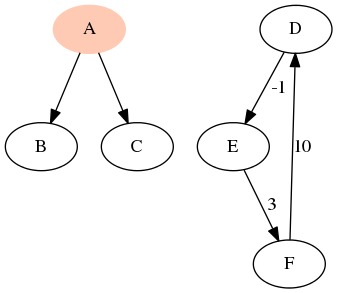
The rendered `firstgraph.dot`
What did that terminal command do? The dot utility is used for producing an image corresponding to a directed graph. (If you want to create the diagram for an undirected graph, consider using neato, or the other variants listed in man dot.) The -Tpng flag will produce PNG output image output, and -o firstgraph.png provides the output name. If you don’t include the -o flag, dot will send its output straight to stdout, which will produce a lot of garbage on the terminal.
Creating a DOT File with Python
Most recently, I used Graphviz to depict the output of a graph coloring (approximation) algorithm within the register allocation routine for a compiler. I wanted to make sure that each pair of adjacent nodes never shared the same color; looking at an adjacency list and checking the coloring by hand would have been difficult; however, by having my program create a DOT file describing the graph coloring, I can check the results at a glance:
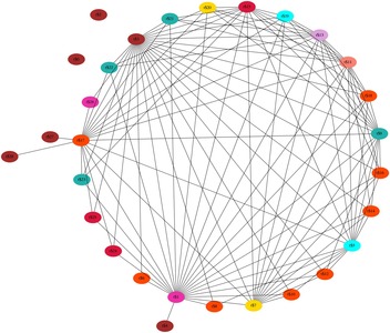
Register interference graph (compiled with circo)
This only required a few lines of Python code (see below), but produces very useful debugging information. The below assumes we represent a graph as a dictionary that maps a vertex label to a set of adjacent vertex labels (essentially an adjacency list, but more pythonic), and writes the output to a file named rig.dot.
 1##
 2# export_graph()
 3#   Saves the graph to a dot file
 4#   graph : a mapping of vertices to sets of vertices
 5#           (adjacency map form)
 6##
 7def export_graph(graph, color=None):
 8  # Map integer colorings to graphviz colors
 9  cmap = {
10           0 : 'brown',
11           1 : 'maroon2',
12           2 : 'orangered',
13           3 : 'crimson',
14           4 : 'lightseagreen',
15           5 : 'gold',
16           6 : 'cyan',
17           7 : 'plum',
18           8 : 'salmon'
19         }
20
21  with open('rig.dot', 'w') as f:
22    f.write('graph G {\n')
23
24    # For each vertex u in the graph
25    for u in graph.keys():
26      # Add coloring information
27      if color:
28        f.write('  "%s" [color=%s, style=filled];\n' % (u, cmap[color[u]]));
29
30      # For each neighbor v of u, add the edge
31      for v in graph[u]:
32        if (u < v):
33          f.write('  "%s" -- "%s";\n' % (u, v))
34
35    f.write('}\n')
You’ll notice that the shape of the graph above is different than the shape of the first graph I showed. Instead of using dot to produce the output image for this graph, I instead used circo (which attempts to draw the graph using a circular layout) and used a command line argument to ensure nodes wouldn’t overlap. The resulting command was $ circo -Goverlap=scale rig.dot -Tpng -o rig.png.
Conclusion
Graphs are an integral data structure for many computer science problems, yet are usually difficult to represent pictorially. Graphviz can help reduce the amount of effort required to produce valuable debug output. In this post, I’ve provided a short example of the DOT format and some example code to output a graph in DOT form.
For users who want more detailed information on how to use Graphviz, I strongly recommend the DOT User’s Manual and reading the manpage (run $ man dot in the terminal).